Does the value of human life in Russia increase with age and higher levels of education?

Ekaterina A. Zubova

doi:10.3897/popecon.5.e79796

Abstract

Estimates of the value of life, reflecting society’s preferences regarding the choice between safety and money, are key indicators for state management in areas such as healthcare, transport, demographic policy, and environmental protection. This article is a logical continuation of the previous research presenting the initial estimates of the value of life in Russia based on analysis of the revealed preferences about employment in industries associated with high fatality risks. In addition to the previous results, this study provides a new theoretical model explaining the logic of choosing employment considering fatality risks and offers estimates of the value of life across educational and age groups. The empirical part of the paper is based on the RLMS HSE data for the period from 2010 to 2020; the author uses panel regression with random effects. The analysis shows that the average value of life in Russia is 287 million rubles, varying from 241 to 450 million rubles depending on levels of education achieved, and considering age value of life ranges from 329 to 349 million rubles (in those groups for which estimates are significant). Possible explanations for this variability are related to the human capital factor, which changes with age and education level. At the same time, the impact of human capital on the value of life can be both positive and negative.

Keywords

value of life, compensation for risk, human capital, panel data, occupational injuries

JEL codes: I, J, K

Introduction

In conditions of limited resources, decision makers have to make difficult choices regarding the allocation of funding. The validity of such decisions should be supported by considerations of the comparative effectiveness of the alternatives, in particular, the cost-benefit analysis based on their implementation. This approach implies a monetary assessment of costs and benefits, including the value of human life.

The term “value of life” is used in this paper with the same meaning as the concepts of “value of human life” and “value of statistical life” (the latter is most widely used in scientific literature).

The idea of measuring the value of life is an example when the theoretical justification for the introduction of the indicator was justified by practical necessity. Even before the publication of the first studies on this topic, in the late 1940s, similar calculations were carried out by the U.S. corporation RAND (Research and Development), fulfilling strategic orders of the U.S. Government to account for human losses during the Cold War (Banzhaf 2014). Today, the value of statistical life is one of the key indicators used in developed countries to assess the benefits and costs of public policy measures in such areas as environmental protection, health, transport, and many others (Banzhaf 2021; Robinson et al. 2019).

At the moment, an officially approved methodology for calculating economic losses from mortality, morbidity, and disability of the population is used in Russia for similar purposes (Order of the Ministry of Economic Development… 2012). The essence of this methodology is that economic losses from mortality are defined as GDP losses due to a person’s removal from the workforce. The preferences of people are not considered in such calculation.

A similar approach to accounting for losses from mortality of the population in the framework of the cost–benefit analysis has been used and is still used in a number of other countries. Nevertheless, in most developed countries, this approach is becoming less and less popular and is being replaced by estimates of the value of life obtained based on an analysis of the population preferences. In particular, in the USA, most calculations carried out by government departments use estimates obtained considering people’s choices about employment in dangerous industries and occupations (Banzhaf 2021).

There are other approaches to assessing the value of life, including that based on the amount of life insurance death benefit, the amount of compensation to relatives of the deceased specified in regulatory legal acts, or the results of public surveys on the fair value of life. A detailed overview of the main approaches can be found, for example, in the works of (Nifantova and Shipitsyna 2012) and (Zubets and Novikov 2018). Nevertheless, the analysis of the compensating wage differential is currently the most reliable methodology (Bykov 2007; Viscusi and Masterman 2017; Banzhaf 2021).

The calculation of the value of life in Russia using this methodology is presented for the first time in (Zubova 2022a); however, alternative estimates have been presented in a number of previous studies. For example, Andrei Bykov (2007) conducts a systematic analysis of existing estimates of the value of life in the United States and Russia, obtained using various approaches. Based on a comparison of these values, he comes to the conclusion that the estimates of the value of life in Russia, recommended for use in public administration, amount to 30-40 million rubles (in 2007 prices). With adjustment for the consumer price index, these values would amount to about 74-99 million rubles in 2020.

In (Zubets and Novikov 2018), the authors present their own econometric model reflecting the population’s decisions regarding migration between regions and at the country level, taking into account differences in life expectancy and average per capita income. Their estimates of the value of life are in the range from 51.3 to 61.1 million rubles.

This article elaborates two previous studies by Ekaterina Zubova (2022a, 2022b), in which the first estimates of the value of life in Russia were proposed based on the revealed preferences of people regarding compensation for the fatality risk at work. In the article (Zubova 2022a), these estimates were obtained based on the analysis of a cross-sectional sample for 2018 and regarding differentiation of risks across sectors of the economy and professions. The following paper (Zubova 2022b) presents the methodology discussion and provides refined estimates on panel data from 2010 to 2020, which enables accounting for unobservable characteristics affecting wage variation, such as differences in employee productivity.

The contribution of the article is threefold. Firstly, it proposes a new theoretical model reflecting the foundations and logic of calculating the value of life. Secondly, based on panel data for Russia, it analyzes the dependence of the value of life on age, which has long been and still is the subject of controversy in other research papers on this topic. Thirdly, it presents empirical estimates of the value of life across population groups defined by their level of education, which, as will be shown later, is one of the main factors differentiating the value of life.

The paper consists of an introduction, four main sections and a conclusion. In the main part, the author considers the theoretical foundations of value-of-life calculations, proposes a new model of equilibrium in the labour market taking into account the choice between safety and money, conducts a review of related empirical work, and presents estimates of the value of life in Russia depending on age and education levels.

Theoretical framework for calculating the value of life

An approach to estimating the value of life considering people’s willingness to pay for risk reduction, or, equivalently, to accept compensation for increased risk, was presented in the work of the Belgian economist Drèze (1962). A few years later, this issue attracted the attention of the English-speaking community — after the publication of Thomas Schelling’s work The life you save can be your own, in which he first introduced the concept of “the value of statistical life” (Schelling 1968).

A simple theoretical justification for the use of the value of life indicator is determined by the formulas described below (Drèze 1962; Hammitt 2000; Andersson and Treich 2011). Faced with life-threatening choices, individuals maximize expected utility (EU):

EU (p, w) = pu_s (w) + (1 – p)u_d (w),(formula 1)

where p is the probability of staying alive, u_s (w) and u_d (w) are utilities if an individual survives or dies, which depends on the amount of his wealth in each case (w).

The value of life itself is defined as the marginal rate of substitution between life safety and money in accordance with the formula:

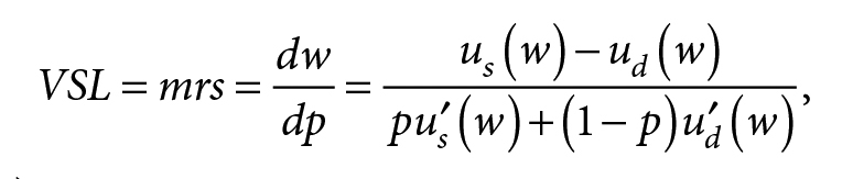(formula 2)

where 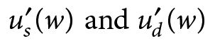are the derivatives of utility functions in terms of wealth (w) if the individual survives or dies, respectively.

The existing approach to determining the value of life as the marginal rate of substitution between life safety and money has several significant drawbacks. Firstly, it takes into account only the marginal change in the amount of risk or the amount of wealth. This circumstance does not allow using this formula for cases when the changes are significant in magnitude. Secondly, it does not account for differences between individuals, including in their attitude to risk and their amount of human capital, whereas empirical studies confirm that there is such a differentiation (see, for example, (Aldy and Smyth 2014; Aldy and Viscusi 2007) on the dependence of the value of life on age).

In addition, this model has weak explanatory power for analyzing the mechanism of risk-related decision-making in the labour market, whereas this context is the most popular in empirical studies (Banzhaf 2021).

It should be noted that, in addition to this specification and its various modifications, there are a number of other, much more complex models in scientific literature that take into account many features of decision-making, including discounting factors, the possibility of accumulating assets, making wills, etc. (see, for example, (Shepard and Zeckhauser 1984; Rosen 1988)). However, more complex models require much more data, which significantly complicates their application for empirical evaluation.

As a compromise between the explanatory power of conceptual foundations and the realism of empirical implementation, a new theoretical model for calculating the value of life based on employment choices and accounting for the risk factor is proposed in the next section.

Theoretical model of equilibrium in the labour market accounting for risk

The theoretical model of employment choice presented below, that regards the differences in the magnitude of the risks of fatal injury by industry, explains the mechanism for determining the value of life.

This model considers a closed economy (there is no labour migration, the supply of labour is fixed) without government intervention. The economy is represented by two industries, in each of which there is one company producing the same product. The product market and the labour market are perfectly competitive. The solution of the model is determined within the framework of the partial equilibrium of labour demand and labour supply, taking into account the fact that workers choose between employment in a “safe” industry for lower wages or in a “risky” industry for a corresponding surplus in pay.

The key consequence of the above-mentioned assumptions of the model is that in terms of making decisions about employment, industries differ only in the magnitude of the risk of death, while other factors affecting the attractiveness of choosing employment in each of the industries do not affect workers.

Consumption sector

Workers (i is the index denoting the reference number of each employee) make employment decisions to maximize the expected utility (EU_i), which is determined by the probability that the employee will survive (pr is the probability of death at work) and his utility from consumption in case of survival:

EU_i = (1 – pr)u_i (c_i, η_i),(formula 3)

where c_i is the volume of consumption of the i-th individual, η_i is a constant reflecting the degree of relative risk aversion by this individual.

The formulation is similar to the model in (formula 1) with the only difference that we assume in advance that the utility in case of death equals zero. This assumption would be unfounded if we believed that employees value bequests, because in the event of their death, relatives can receive compensation. However, since in fact in the labour market, compensation for risk usually is a regular wage surplus, after the death of an employee, their family (except for some cases stipulated in the legislation on compensation to the relatives of the deceased) simply loses this source of income, so that death cannot be considered to bring non-zero utility.

The utility of an individual (u_i) from consumption is expressed by a function with constant relative risk aversion (CRRA), taking into account that the attitude to risk can also vary among individuals:

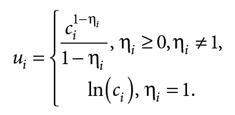(formula 4)

Next, we will omit the limiting case in which η_i = 1 since this is not essential for the conclusions of the model.

The assumption of differences in the degree of risk aversion is difficult to account for in the process of empirical assessment, but it is fundamentally important for understanding reality, since some people (“preferring adventure”) may be more willing to engage in risky work, while others (“preferring tranquility”) value safety significantly higher.

Workers also differ in the amount of human capital (h_i) which affects their productivity. The amount of human capital depends on the level of education (s_i) and the age of the employee (a_i):

h_i = h_i (s_i, a_i),(formula 5)

The dependence of the amount of human capital on the level of education achieved is more likely to be positive, but the relationship with age is less unambiguous. This dependence can be non-linear, since, on the one hand, over the years, a person gains experience and develops certain skills, but, on the other hand, as they age, physical abilities may deteriorate, and productivity may decrease.

In the absence of the possibility of borrowing and savings, as well as any sources of income other than labour income, a one-period budget constraint takes the following form:

c_i = w_i,(formula 6)

where w_i is the wage of the i-th employee.

Production sector

The task of firms is to maximize profits. The sphere of production is represented by two industries (j is the number of the industry, j = {1,2}). Output in each industry is described by the Cobb-Douglas production function and depends on the level of technological progress (A), the amount of physical capital (K), the number of employees (L) and the average level of human capital per employee (H). For simplicity, we assume that the marginal cost of renting capital and the depreciation rate are zero, since this premise does not lead to a limitation of the generality of results in terms of calculating the value of life. Thus, the marginal costs of firms are related only to labour costs, and the output function looks as follows:

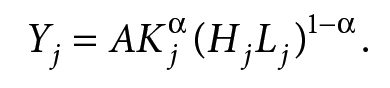(formula 7)

Each of the industries employs L_j workers, each of whom has a certain level of human capital:

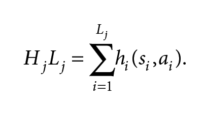(formula 8)

All firms are risk-neutral. Industries differ in the probability of death of an employee at work, depending on whether firms in this industry incur additional costs (v) to ensure occupational safety. By introducing such a distinction, we assume that in the real economy, firms can potentially reduce the risk to the lives of employees to zero if they make the necessary investments in ensuring safety at the workplace. Since the cost of such investments can be substantial, it is not profitable for firms to invest if employees agree to take on the risk in exchange for monetary compensation, the amount of which is less than the estimated cost of the necessary investments.

In the first industry (j = 1), the risk of death at work is zero, and the marginal costs for each employee (mc_ij) are the sum of his wage (w_ij) and the costs associated with ensuring occupational safety per employee (v > 0):

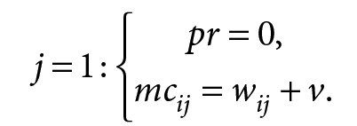(formula 9)

In the second industry (j = 2), the risk of death at work is greater than zero (but less than one, since we do not consider the marginal case in which the probability of the death of an employee is 1, because in the absence of the value of bequests, it makes no sense to agree to imminent death for any amount of money), and firms do not incur additional safety costs:

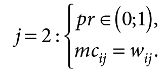(formula 10)

Balance of labour demand and labour supply

Within the framework of this model, it is assumed that each employee is employed in one of the industries. The marginal product of a unit of labour (one worker) per unit of human capital is equal to the partial derivative of the expression given by formula 7, with respect to (H_jL_j):

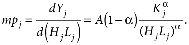(formula 11)

The balance of supply and demand for labour in each of the industries implies equality of the marginal product of labour provided by a certain level of human capital (mp_j × h_i (s_i, a_i)) to marginal costs of firms per employee (mc_ij in formulas 9 and 10):

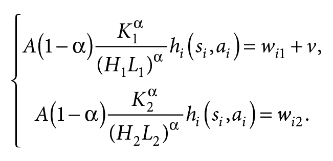(formula 12)

Thus, an employee’s salary in a “safe” industry, other things being equal (including with an equal level of human capital), will be lower than in a “risky” industry due to the deduction of labour safety costs (which is similar to the situation when a risk premium equal to v is introduced in a dangerous industry).

According to the definition of the value of life accepted in scientific literature, it is equal to the marginal rate of substitution between safety of life with money. For each employee, this parameter is calculated using the following formula:

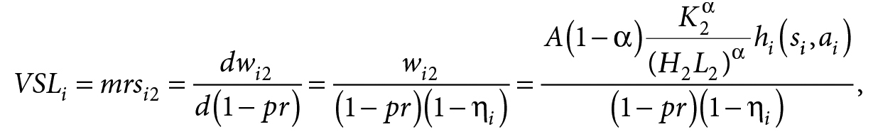(formula 13)

Thus, the value of life positively depends on the amount of human capital and the degree of employee’s risk aversion. It is important to note that such an approach to estimating the value of life is valid only for the extreme case when we assume that the probability of death in a relatively risk-free situation increases by a small amount. If the difference in risk is large, the use of the marginal substitution rate is irrelevant. In this case, it would be more correct to estimate the value of life as the amount of “fair compensation”, that is, satisfying workers in terms of expected utility, for the probability of death close to 1.

To determine fair compensation, we consider a situation in which employees do not care which industry they work in, since in both cases they expect the same level of utility. Equality of expected utilities in the case of zero (j = 1) and non-zero (j = 2) risk is determined by the following expression:

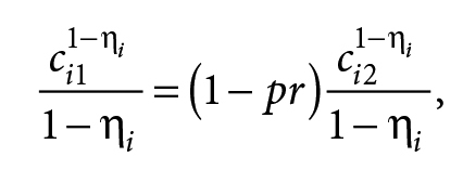(formula 14)

Since, in accordance with the budget constraint, the level of consumption is equal to the amount of wages, we can represent the expression from formula 14 as follows:

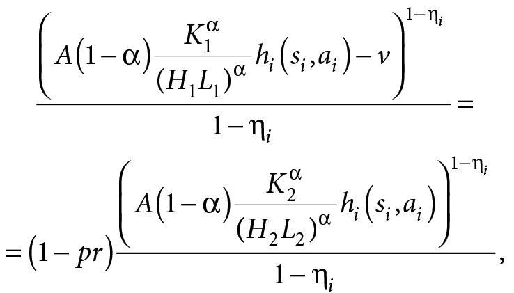(formula 15)

By converting this expression, we can determine the “fair” value of the risk premium:

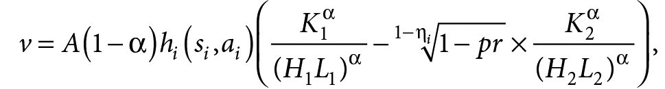(formula 16)

This value reflects the amount of the minimum allowance at which the employee agrees to choose a risky job. Thus, the value of this premium increases as the level of human capital (based on age and education level) increases, as the degree of risk increases, and as the employees’ risk aversion increases.

In addition, this value also depends on the decisions made by other individuals, since they are responsible for the distribution of labour and human capital between the two industries, and, accordingly, for the demand for labour in each of the industries. The more labour and human capital involved in a “risky” industry and the less in a “safe” one, the higher the premium should be. The meaningful interpretation is that the more workers there are in the industry and the higher the amount of human capital involved, the smaller the marginal product that falls on each additional employee and unit of their human capital, and the lower their resulting wage.

This model illustrates the basic economic intuition behind the term value of life within the framework of the use of the compensating wage differential methodology: employees can choose whether to accept additional risk for an appropriate compensation or to work in a safer, but lower-paying job. In addition, the interpretation of this situation is also given above by firms: theoretically, they could minimize the risks of occupational injuries by spending additional resources on improving working conditions, but in terms of costs, it may be more profitable to simply pay employees an appropriate compensation.

At the same time, considering the above-mentioned prerequisites, this model has several significant limitations. One of the key among them is that industries or firms differ only in the level of risk. Obviously, in reality, the differences between industries and types of work within them are much wider, which, of course, will affect both the attractiveness of choosing employment in a particular industry for employees, and the amount of wages offered to them. This may concern not only working conditions, but also the requirements imposed on employees, which calls into question the premise of perfect competition in the labour market. For example, competition between workers with high and low levels of education may be far from perfect, since certain types of work (for example, in the field of education or high technology) may be available only to people with higher education, so in some sense this partly gives them monopoly power, as a result of which the wages offered to them will be higher even in the absence of risk.

In addition, in terms of applicability to reality, the premise of a closed economy and the absence of labour migration may play an important role, since labour migrants (primarily working illegally) may be forced to engage in more dangerous work even in the absence of fair compensation for risk due to the fact that their choice regarding employment is limited.

Another important point is the use of a simple one-period budget constraint. In real life, employment decisions can be influenced by the presence of a discounting factor, as well as the availability of other sources of income, the availability of borrowing and savings, etc. All these factors create the need for an intertemporal choice, the results of which may differ significantly from a single-period specification.

Despite all the limitations listed above, within the framework of this model, the main task was to reflect the essence of the choice regarding employment considering the risk factor, while further improvements can serve as directions for future research in this area.

Review of empirical background

The most significant contribution to the empirical assessment of the value of life belongs to the U.S. economist William Viscusi. In his works and in collaboration with other scientists, he proposed and continues to develop the most popular methodology for assessing the value of life based on determining people’s willingness to accept risky work for appropriate compensation in wages (see, for example, (Viscusi 1993, 2004, 2011; Viscusi and Aldy 2003; Viscusi and Masterman 2017), etc.).

According to the methodology proposed by Viscusi (2004), the value of life is calculated in two stages. At the first stage, the hedonic wage regression equation is estimated, where the probability of fatal injury at work is used as a variable of interest:

(formula 17)

where wage_i is the hourly wage rate of an employee with index i, X_i is the vector of control variables, β, γ₁, γ₂ are regression coefficients, ε_i is idiosyncratic shock.

At the second stage, the death risk coefficient (γ₁) is used to calculate the value of life directly according to the following formula:

(formula 18)

where average wage is the average hourly wage in the sample, is the estimate of the coefficient for fatality risk in production from the equation of formula 17, the number of deaths is calculated per 100,000 people, the duration of the working year is taken as 2,000 working hours.

In another paper, Kniesner et al. (2012) proposed an adaptation of this approach to the analysis of panel data, which, according to the results of their research, enables significantly refining estimates of the value of life, including reducing their confidence intervals by accounting for unobservable characteristics. Comparing the values obtained based on the analysis of cross-sample and panel data, the authors concluded that in the first case, the estimates are unreasonably overestimated due to omitted variables bias, the effect of which can be reduced by the use of individual and time effects in panel models. Their approach will be described in more detail below, as it is used in the empirical part of this article.

In addition to individual studies on the value of life, meta-analyses have become increasingly popular in recent years (see, for example, (Murphy et al. 2005; Doucouliagos et al. 2012; Doucouliagos et al. 2014)). This approach enables aggregating the results of previous studies and verifying the reliability of the obtained estimates. Since quite a lot of similar studies have also appeared today, a new level of generalization suggests a “meta-meta-analysis” presented in the Banzhaf article (2021). As the author of this paper notes, one of the key drawbacks of existing estimates of the value of life, in hedonic wage studies, is ignoring age as a factor of differentiation of such estimates.

A partial analysis of the dependence of the value of life on age was carried out in (Aldy and Smyth 2014; Aldy and Viscusi, 2007, 2008). The authors of the research came to the conclusion that the value of life either decreases with age, or has the form of an inverted U-shaped curve, steadily increasing until a certain age, and then starting a slow decline. Although these results are consistent with considerations about the dynamics of income and consumption within the life cycle, they still require proof of external validity. In addition, this pattern was defined for the U.S. data and is not necessarily observed for other countries.

In the empirical part of the study presented in the next section, the dependence of the value of life on age is tested on Russian data. In addition, the author analyzes the relationship with education, seeing it as another crucial factor affecting the amount of human capital.

Estimation of the value of life in Russia considering age and educational level

The empirical calculations presented below are based on the approach traditionally used in foreign studies to estimate the value of life based on the compensating wage differential and economic intuition, following from the theoretical model described above. As can be seen from table 1 with descriptive statistics, the maximum number of deaths is 24 per 100,000 people. This risk can be considered relatively small, so the calculation of the value of life as the marginal rate of substitution between safety of life and money will be correct. In addition, dividing the sample into subgroups by age and level of achieved education enables testing theoretical conclusions about the relationship between the value of life and the amount of human capital.

Data and methodology

Calculations are carried out on the data of the Russian Longitudinal Monitoring Survey (hereinafter referred to as the HSE RLMS) for the period from 2010 to 2020. The author uses a representative individual sample and draws the observations having complete information on the following parameters:

wages,
belonging to a certain employment industry and professional group (in the HSE RLMS data, the professional group reflects the level of qualifications: from unskilled workers in all industries to legislators, senior officials, senior and middle managers),
gender, age, marital status, region of residence.

By analogy with foreign papers on this topic, only working individuals with non-zero wages are considered, and the missing values are ignored.

The risks of fatal and non-fatal injuries in the workplace are calculated according to the Rosstat Bulletin Industrial injuries in the Russian Federation as the ratio of the number of occupational injuries in each specific industry to the total number of people employed in this industry per 100,000 people.

Table 1 presents descriptive statistics of the data used for calculations. The structure of the sample by region of residence and occupational groups, which are used as control variables, is not given due to the large number of categories.

Table 1.

Download as

CSV

XLSX

Descriptive statistics

Variable	Average value	Standard deviation	Median	Minimum value	Maximum value
Wage (rubles per hour)	93.90	71.83	78.51	0.085	2463.56
Age (years)	40.81	12.2	40.0	14.0	87.0
Risk of fatal injury at work (number of deaths per 100,000 workers in the industry)	5.565	5.63	4.62	0.0	24.0
Risk of non-fatal injury at work (number of non-fatal injuries per 100,000 workers in the industry)	108.33	83.535	93.76	0.0	452.0
Categorical variables (share in the total number of observations)
Gender	0 — men			1 — women
Gender	0.443			0.557
Distribution by level of education	Incomplete secondary	Secondary general	Vocational training school	Technical school	Higher
Distribution by level of education	0.06	0.11	0.21	0.24	0.38
Distribution by age groups	Under 25	25–34	35–44	45–54	Older than 54
Distribution by age groups	0.08	0.27	0.27	0.22	0.16
Marital status	Never married	Married	Live together, not registered	Divorced	Widow or widower
	0.13	0.59	0.14	0.09	0.05
	The marriage is registered, but spouses do not live together		Did not answer the question
	less than 0.01

Panel data enable accounting for important unobservable factors affecting wage variation as individual and time effects. In terms of individual, time-invariant characteristics, one of these factors is most likely labour productivity. Time effects correct the influence of general dynamic trends, in particular structural fluctuations in the labour market.

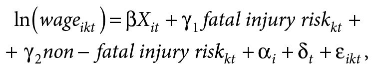
As it was shown in (Kniesner et al. 2012), the use of panel data to calculate the value of life allows for more accurate estimates compared to cross-sample analysis. In this article, the author uses a similar regression model with individual and time effects:

(formula 19)

where wage_ikt is the rate of hourly wage of a worker with index i, employed in industry k in year t, X_it is the vector of control variables (age, age squared, gender, education level, region of residence, marital status, occupational group), fatal injury risk_kt and non – fatal injury risk_kt are the risk of fatal and non-fatal injury to the production in industry k in year t accordingly, α_i is the individual effect, δ_t is the time effect, ε_ikt is idiosyncratic shock.

In (Kniesner et al. 2012) for the USA and (Zubova 2022b) for Russia, several panel model specifications are considered, including those with random and fixed effects. The model with fixed effects is significantly better suited for solving the problem of accounting for unobservable characteristics, primarily labour productivity, since this parameter can correlate both with wages and with the choice of employment in a particular industry. Nevertheless, as it was shown in (Zubova 2022b), the use of a model with fixed effects leads to that most observations are not actually considered in the calculations, since the fatality risk variation is important for determining the coefficient for the risk variable. Basically, this coefficient is determined by “marginal” individuals who have moved from a more dangerous industry to a less dangerous one within the given period, or vice versa, since in other cases the variation of the risk variable over time is too small.

Due to differences in the number of observations and the number of variables, some of which also fall out due to the lack of variation over time, it is incorrect to choose among models with different types of effects based on statistical tests (for example, the Hausman test). It is possible to compare estimates using both types of effects on a complete sample, as it was shown in Zubova’s work (2022b). In the models with fixed effects, the coefficient estimates for the risk of fatal injury turned out to be lower than in those with random effects (7 · 10^–3 vs 8 · 10^–3, respectively); however, these estimates are quite close in magnitude and significantly lower than in other specifications not accounting unobservable effects (12 · 10^–3). Our interest is in estimating the value of life across educational and age groups, which stand for parts of the total sample, and that means a significantly smaller number of observations, so a possible increase in the accuracy of estimates due to the use of fixed effects does not justify the loss of a significant part of observations due to the limitations of using models of this type. Therefore, in this paper, the choice is made in favour of random effects.

Division into educational groups was carried out in accordance with the main stages of education: incomplete secondary education, secondary general education, vocational training school, technical school, and higher education. Age groups are represented by ten-year intervals with the exception of the youngest and oldest ones. The youngest group includes individuals from 18 to 24 years old, as this is usually the age when young people do not yet have a full education and are forced to combine work with study. The oldest group includes individuals who have reached 55 years of age and older, that is, in pre-retirement and retirement ages.

Results

Table 2 presents the results of estimating the regression of the logarithm of wages with random effects on the full sample and on the subsamples for five educational groups.

Table 2.

Download as

CSV

XLSX

Estimation of hedonic wage regression across educational groups

	Total sample	Incomplete secondary	Secondary general	Vocational training school	Technical school	Higher
Constant	3.445***	4.136***	3.993***	4.207***	3.97***	3.897***
Constant	(1.043)	(0.43)	(0.356)	(0.251)	(0.229)	(1.9)
Age	0.034***	0.036**	0.035***	0.035***	0.066***	0.06***
Age	(0.004)	(0.016)	(0.013)	(0.009)	(0.005)	(0.007)
Age ²	-0.001***	-0.001***	-0.001***	-0.001***	-0.001***	-0.001***
Age ²	(0.0001)	(0.0002)	(0.0001)	(0.00005)	(0.00002)	(0.0001)
Gender (female = 1, male = 0)	-0.341***	-0.334***	-0.302***	-0.355***	-0.332***	-0.337***
Gender (female = 1, male = 0)	(0.021)	(0.085)	(0.067)	(0.047)	(0.004)	(0.032)
Risk of fatal injury	0.008***	0.016**	0.008	0,01**	0,009**	0,006*
Risk of fatal injury	(0.002)	(0.007)	(0.005)	(0.003)	(0.004)	(0.003)
Risk of non-fatal injury	0.0002	0.0002	0.0003	0.0002	0.0002	0.0002
Risk of non-fatal injury	(0.0001)	(0.0005)	(0.0004)	(0.0002)	(0.0003)	(0.0002)
Control for marital status	yes	yes	yes	yes	yes	yes
Control for the region of residence	yes	yes	yes	yes	yes	yes
Control for the level of education	yes	_	_	_	_	_
Control for professional groups	yes	yes	yes	yes	yes	yes
Time/Individual effects	yes/yes	yes/yes	yes/yes	yes/yes	yes/yes	yes/yes
Adjusted R²	0.455	0.437	0.449	0.455	0.445	0.399
Number of observations	73,785	4,093	8,165	15,760	17,947	27,820

Based on the coefficients for the death risk variable from Table 2, we calculate the value of life (see Table 3). The coefficient for the risk variable decreases with the level of education, while the average wage, on the contrary, increases. However, in terms of the value of life, wage growth is slower, and it cannot compensate for the decrease in risk, so the value of life decreases as the level of education increases. At the same time, for a group of people with secondary general education, the risk coefficient is not significant, which may be due to the small number of observations in this category associated with risky work. The group of people with higher education is the largest, and we see that the value of life in this group in Russia is significantly lower than that typical for people with incomplete secondary education.

Table 3.

Download as

CSV

XLSX

Estimates of the value of life across educational groups

	Total sample	Incomplete secondary	Secondary general	Vocational training school	Technical school	Higher
Average wage per hour, in rubles	93.89	77.31	81.78	81.58	81.12	115.09
Coefficient for fatal injury	0.00838	0.015935	not significant	0.010033	0.009203	0.005731
Value of life, in rubles (in 2010 prices)	157,359,640	246,386,970	-	163,698,428	149,309,472	131,916,158
Value of life, in rubles (in 2020 prices)	287,436,644	450,055,960	-	299,015,216	272,732,027	240,961,010

Similarly to the analysis by educational groups, table 4 presents estimates of the regression of the natural logarithm of wages across age groups.

The fatality risk coefficients from table 4 allow for the calculation of the value of life by age groups presented in table 5. As can be seen from the last two columns, coefficient estimates are not significant for people over the age of 45, so the value of life cannot be calculated. This is probably due to the fact that at older ages people are less likely to engage in risk-related work for health reasons. Nevertheless, the estimate of the value of life for the full sample is significantly lower than in any of the groups up to 44 years old, thus, we can conclude that the older groups put downward pressure on it.

The values calculated based on this methodology may be biased upwards since they are not adjusted for the presence of unobservable factors of variation in the form of fixed effects. However, these differences are relatively small and fall within the margin of error, and the estimates can be considered fairly accurate.

As shown in (Zubova 2022a), estimates of the value of life based on the compensating differential are significantly higher than any other estimates previously obtained for Russia using a different methodology, both with stated (2.4–13.3 million rubles in 2019 prices) and revealed (51.3–131.8 million rubles in 2017 prices) preferences. Similarly, the values obtained in this study are higher than those proposed by Bykov (2007) based on a review of alternative approaches (30–40 million rubles in 2007 prices or approximately 74–99 million rubles when adjusted to the dynamics of the CPI up to 2020) and by Zubets and Novikov (2018) within their own econometric model (51.3–61.1 million rubles). They are also significantly higher than the amount of compensation to relatives of people who died under certain circumstances, fixed in legislative acts of the Russian Federation and court decisions: from 0.5 to 9.2 million rubles according to the results of the analysis carried out in (Zubets and Novikov 2018).

On the other hand, in comparison with the alternative estimates listed above, the results of this paper are closest to the official estimates of government departments and empirical works in the USA (11.4 million US dollars in 2020 prices according to data of the U.S. Department of Health and Human Services; according to the results of the analysis in Banzhaf (2021), the average estimate was $6.98 million in 2019 prices). In both cases, estimates for the United States were obtained using a methodology comparable to the approach used in this paper, which, as mentioned above, is by far the most reasonable. A detailed comparison of estimates and discussion of possible differences in the structure of risks between the United States and Russia is also presented in (Zubova 2022a).

Table 4.

Download as

CSV

XLSX

Estimation of hedonic wage regression across age groups

	Total sample	Under 25	25–34	35–44	45–54	Older than 54
Constant	3.445***	-2.806	3.972**	3.413	4.013	5.864***
Constant	(1.043)	(2.637)	(1.493)	(2.419)	(3.453)	(2.474)
Age	0.034***	0.588**	0.008	0.022	0.043	-0.009
Age	(0.004)	(0.217)	(0.068)	(0.091)	(0.129)	(0.058)
Age ²	-0.001***	-0.012*	-0.001	-0.0002	-0.0001	-0.0002
Age ²	(0.0001)	(0.005)	(0.0001)	(0.001)	(0.001)	(0.0004)
Gender (female=1, male=0)	-0.341***	-0.306***	-0.405***	-0.391***	-0.297***	-0.233***
Gender (female=1, male=0)	(0.021)	(0.054)	(0.032)	(0.041)	(0.053)	(0.065)
Risk of fatal injury	0.008***	0.012*	0.01***	0.009*	0.006	0.006
Risk of fatal injury	(0.002)	(0.005)	(0.003)	(0.003)	(0.004)	(0.005)
Risk of non-fatal injury	0.0002	0.0002	-0.00003	-0.00005	0.0003	0.0003
Risk of non-fatal injury	(0.0001)	(0.0004)	(0.0002)	(0.0002)	(0.0002)	(0.0003)
Control for the level of education	yes	yes	yes	yes	yes	yes
Control for marital status	yes	yes	yes	yes	yes	yes
Control for the region of residence	yes	yes	yes	yes	yes	yes
Control for professional groups	yes	yes	yes	yes	yes	yes
Time/Individual effects	yes/yes	yes/yes	yes/yes	yes/yes	yes/yes	yes/yes
Adjusted R²	0.455	0.369	0.402	0.484	0.497	0.475
Number of observations	73,785	6,010	20,304	19,558	16,281	11,632

Table 5.

Download as

CSV

XLSX

Estimates of the value of life across age groups

	Total sample	Under 25	25–34	35–44	45–54	Older than 54
Average salary per hour, in rubles	93.89	82.62	100.45	102.98	91.63	76.08
Coefficient for fatal injury	0.00838	0.011567	0.009849	0.008755	not significant	not significant
Value of life, in rubles (in 2010 prices)	157,359,640	191,133,108	197,866,410	180,317,980	_	_
Value of life, in rubles (in 2020 prices)	287,436,644	349,128,018	361,427,218	329,372,863	_	_

Conclusion

As the practice of public administration in many developed countries shows, the value of life is the most important parameter for cost–benefit analysis of public policy measures. Particularly, in the USA, these estimates are calculated at the official level and are published on the official websites of government departments (see, for example, (U.S. Department of Health and Human Services 2021; U.S. Department of Transportation 2021; U.S. Office of Management and Budget 2003)). The introduction of the practice of calculating and using such estimates in the Russian Federation should contribute to improving the quality of public administration in terms of policy planning, as well as allowing the use of a methodology comparable with other countries for analyzing the comparative effectiveness of government programmes.

This article presents a new theoretical model explaining the mechanism of choice in the labour market considering fatality risks. The contribution to the development of the methodology for estimating the value of life is that this model enables understanding the economic logic of the formation of this indicator and can be used to explain the results of empirical calculations. In addition, the use of parameters such as the amount of human capital and the degree of risk aversion in the model provides grounds for further research, which should enable clarifying existing estimates.

The empirical part of the paper presents calculations of the value of life in Russia across educational and age groups. The results of the analysis by age groups generally confirm the studies based on the U.S. data and show that the dependence of the value of life on the age is nonlinear, that is, the indicator increases up to a certain period, and then begins to decrease. At younger ages, these changes may be associated with an increase in human capital due to the acquisition of experience, knowledge, and skills, which is consistent not only with the general results of other studies on this topic, but also with the logic proposed within the framework of the developed theoretical model. At the same time, the decrease in the value of life in the group aged 35 to 44 years old and statistical insignificance of the estimates for older age groups most likely indicate that with age people are less inclined to engage in risky work or receive an insignificant increase in wages for this. Firstly, due to the deterioration of health, as well as the accumulation of knowledge and experience that open up a wider choice of employment in safe industries, risky work may become less attractive with age. Secondly, an increase in the likelihood of occupational injuries for health reasons can lead to a decrease in productivity, and, accordingly, competitiveness in the labour market in risk-related industries.

The analysis of the value of life across educational groups, to the author’s knowledge, is carried out in this study for the first time. However, the calculations show that this factor is even more significant for explaining the differentiation of the value of life than age. The death risk coefficient and the average wage are negatively correlated, but the deviation of coefficients is significantly larger, which leads to a decrease in the value of life with an increase in the level of education. Although this result contradicts the logic of the theoretical model, it is most likely due to the decline in the prevalence of risky professions among people with higher education. A possible interpretation is that people with a higher level of education, other things being equal, have greater opportunities to receive decent wages without putting their lives at risk, and those of them who choose risky professions are characterized by a lower degree of risk aversion (in the theoretical model, we conditionally called them “preferring adventure”).

Literature

Aldy JE, Smyth SJ (2014) Heterogeneity in the Value of Life. National Bureau of Economic Research Working Paper Series 20206. https://doi.org/10.3386/w20206

Aldy JE, Viscusi WK (2007) Age Differences in the Value of Statistical Life: Revealed Preference Evidence. Review of Environmental Economics and Policy 1(2): 241-60. URL: https://scholar.harvard.edu/jaldy/publications/age-differences-value-statistical-life-revealed-preference-evidence

Aldy JE, Viscusi WK (2008) Adjusting the Value of a Statistical Life for Age and Cohort Effects. Review of Economics and Statistics 90(3): 573-81. URL: https://scholar.harvard.edu/jaldy/publications/adjusting-value-statistical-life-age-and-cohort-effects

Andersson H, Treich N (2011) The Value of a Statistical Life. In: de Palma AR, Quinet LE, Vickerman R (Eds) Handbook in Transport Economics. Edward Elgar, Cheltenham, UK, 396-424. URL: https://www.tse-fr.eu/sites/default/files/medias/doc/by/andersson/andersson_treich_handbook_vsl_chapter_2011.pdf

Banzhaf HS (2014) Retrospectives: The cold-war origins of the value of statistical life. The Journal of Economic Perspectives 28(4): 213–26. http://dx.doi.org/10.1257/jep.28.4.213

Banzhaf HS (2021) The value of statistical life: A meta-analysis of meta-analyses. National Bureau of Economic Research Working Paper Series 29185. https://doi.org/10.3386/w29185

Bykov AA (2007) On methodology for economic assessment of the value of statistical life (explanatory note). Problems of Risk Analysis 2. URL: https://cyberleninka.ru/article/n/o-metodologii-ekonomicheskoy-otsenki-zhizni-srednestatisticheskogo-cheloveka-poyasnitelnaya-zapiska (in Russian)

Doucouliagos C, Stanley TD, Giles M (2012) Are estimates of the value of a statistical life exaggerated? Journal of Health Economics 31(1): 197-206. http://dx.doi.org/10.1016/j.jhealeco.2011.10.001

Doucouliagos H, Stanley TD, Viscusi WK (2014) Publication selection and the income elasticity of the value of a statistical life. Journal of Health Economics 33(1): 67–75. http://dx.doi.org/10.1016/j.jhealeco.2013.10.010

Drèze JH (1962) L’Utilité Sociale d’une Vie Humaine. Revue Française de Recherche Opérationnelle 6: 93–118. URL: http://hdl.handle.net/2078.1/86717

Hammitt JK (2000) Valuing mortality risk: Theory and practice. Environmental Science and Technology 34(8): 1396–1400. https://doi.org/10.1021/es990733n

Kniesner TJ, Viscusi WK, Woock C, Ziliak JP (2012) The value of a statistical life: Evidence from panel data. The Review of Economics and Statistics 94(1): 74–87. https://doi.org/10.1162/REST_a_00229

Murphy JJ, Allen PG, Stevens TH, Weatherhead D (2005) A meta-analysis of hypothetical bias in stated preference valuation. Environmental and Resource Economics 30: 313–25. https://doi.org/10.1007/s10640-004-3332-z

Nifantova RV, Shipitsina SE (2012) Modern methods of human life evaluation. Economy of regions 3. URL: https://cyberleninka.ru/article/n/sovremennye-metodicheskie-podhody-v-otsenke-stoimosti-chelovecheskoy-zhizni (in Russian)

Robinson LA, Hammitt JK, O’Keeffe L (2019) Valuing Mortality Risk Reductions in Global Benefit-Cost Analysis. Journal of Benefit-Cost Analysis 10(S1): 15-50. http://dx.doi.org/10.1017/bca.2018.26

Rosen S (1988) The Value of Changes in Life Expectancy. Journal of Risk and Uncertainty 1(3): 285–304. URL: https://www.jstor.org/stable/41760544

Schelling TC (1968) The life you save may be your own. In: Chase SB (Ed.) Problems in public expenditure analysis. Studies of government finance. The Brookings Institution, Washington, DC, USA, 127–62.

Shepard DS, Zeckhauser RJ (1984) Survival versus Consumption. Management Science 30(4): 423–39. URL: https://www.jstor.org/stable/2631430

Viscusi WK (1993) The Value of Risks to Life and Health. Journal of Economic Literature 31(4): 1912–46. URL: https://www.jstor.org/stable/2728331

Viscusi WK (2004) The value of life: Estimates with risks by occupation and industry. Economic Inquiry 42(1): 29–48. https://doi.org/10.1093/ei/cbh042

Viscusi WK (2011) What’s to know? Puzzles in the literature on the value of statistical life. Vanderbilt Law and Economics Research 11-36. https://dx.doi.org/10.2139/ssrn.1908376

Viscusi WK, Aldy JE (2003) The Value of a Statistical Life: A Critical Review of Market Estimates throughout the World. Journal of Risk and Uncertainty 27: 5-76. URL: https://www.jstor.org/stable/41761102

Viscusi WK, Masterman C (2017) Income elasticities and global values of a statistical life. Journal of Benefit-Cost Analysis 8(2): 226–50. http://dx.doi.org/10.1017/bca.2017.12

Zubets AN, Novikov AV (2018) Quantitative assessment of the value of human life in Russia and in the world. Finance: Theory and Practice 22(4): 52–75. https://doi.org/10.26794/2587-5671-2018-22-4-52-75 (in Russian)

Zubova ЕА (2022a) Value of statistical life in Russia based on microdata. Journal of the New Economic Association 1 (53): 163–179. DOI: 10.31737/2221-2264-2022-53-1-8 (in Russian)

Zubova ЕА (2022b) Value of statistical life in Russia: Estimates based on panel microdata for 2010–2020. Applied Econometrics 65: 45-64. DOI: 10.22394/1993-7601-2022-65-45-64 (in Russian)

Other data sources

Order of the Ministry of Economic Development of Russia No. 192, Ministry of Health and Social Development of Russia No. 323n, the Ministry of Finance of Russia No. 45n, Rosstat No. 113 (2012) “On approval of the Methodology for calculating economic losses from mortality, morbidity and disability of the population” of 10.04.2012 (Registered with the Ministry of Justice of Russia on 28.04.2012 No. 23983) https://rg.ru/pril/73/43/77/23983_metodologiia.pdf (in Russian)

U.S. Department of Health and Human Services (2021) Updating value per statistical life (VSL) estimates for inflation and changes in real income. https://aspe.hhs.gov/sites/default/files/2021-07/hhs-guidelines-appendix-d-vsl-update.pdf

U.S. Department of Transportation (2021) Treatment of the value of preventing fatalities and injuries in preparing economic analyses. https://www.transportation.gov/resources/value-of-a-statistical-life-guidance

U.S. Office of Management and Budget (2003) Circular A-4. https://www.whitehouse.gov/sites/whitehouse.gov/files/omb/circulars/A4/a-4.pdf

Information about the author

Zubova Ekaterina Andreevna, Fox Fellow (2021-2022) at Yale University, New Haven, Connecticut, 06511, USA. Email: ekaterina.zubova@yale.edu